Parameter Optimization
In Machine Learning, "Training" is essentially a search game. We are looking for the "Magic Numbers" ( weights ) ( and ) ( biases ) that allow our math formula to predict the future correctly.
1. The Goal: Defining the Cost Function
Before we can "optimize" (improve) anything, we need to mathematically define what "bad" looks like. We call this the ( Cost ) ( Function ).
The Logic Flow: From Model to Cost
Step 1: The Prediction ($Y'$)
We pick some random random values for our parameter $\theta$ (weight) and $b$ (bias).
$ Y' = \theta \cdot X + b $
Step 2: The Comparison (Error)
We compare our prediction ($Y'$) against the actual answer ($Y$) to see how far off we are.
$ \text{Error} = Y' - Y $
Step 3: The Cost ($J$)
We cannot just add up the errors (negatives) (would) (cancel) (positives). So we square them and take the average.
This final number—the "Average Squared Error"—is what we call the Cost Function $J(\theta)$.
The Optimization Goal: Changing the weights ($\theta$) to find the specific value that makes $J(\theta)$ as small as possible.
2. The Solutions: How to Minimize $J(\theta)$
Now that we defined the problem (The) (Cost) (Function), we need a method to solve it. There are two main ways to find the bottom of this valley.
Method A: Ordinary Least Squares
For Linear Regression, there is a "Magic Formula" that calculates the perfect weights instantly, without any guessing. This is the Normal Equation.
- Pros: Finds the exact optimal solution instantly. No "learning rate" needed.
- Cons: Requires inverting a matrix ($X^T X$). If you have 1,000,000 features, this is computationally impossible (slow).
The Normal Equation is $O(n^3)$. If you double your features, the calculation time increases by 8x.
For small datasets (e.g., 100 features), OLS is great. For modern "Big Data" (100,000+ features or Neural Networks), OLS crashes computers. That is why we need Gradient Descent.
Method B: Gradient Descent (The Iterative "Walk")
👉 Click here for a Step-by-Step "Mountain Analogy" Explanation
When we can't solve the formula directly (most ML/Deep Learning models), we use an iterative approach.
Visualizing Gradient Descent
The curve is the Cost Function (Error). The Ball is our Model.
Current Slope: --
Key Concepts:
- Gradients: The "slope" of the hill. It points Up, so we go the opposite direction.
- Learning Rate ($\alpha$): Size of the step.
- Too small: Takes forever.
- Too big: Overshoots the bottom and might diverge.
Variants of Gradient Descent:
3. The Shape of the Cost Function ( Convexity )
If we have a model with 2 parameters (e.g., Slope $m$ and Intercept $b$), the Cost Function becomes a 3D Surface (a Bowl).
3D Cost Surface ( Convex Bowl )
X & Z Axes: Parameters ( $\theta_0, \theta_1$ ) | Vertical Y Axis: Error ( $J$ )
What about more parameters?
If we have 100 features, the graph becomes a Hyper-Paraboloid (101 dimensions). We can't draw it, but the math tells us it keeps this same "Bowl" shape.
Because Linear Regression's cost function is always a "Bowl" (Convex), there is only one lowest point (Global Minimum). Gradient Descent is guaranteed to find it!
4. The Challenges of Optimization
Knowing the math is one thing; making it work in practice is another. Here are the two biggest hurdles you will face.
A. Choice of Learning Rate ($\alpha$)
This is the "Goldilocks" problem.
- Too Small: You will reach the bottom, but it might take 1,000,000 steps. (Inefficient)
- Just Right: Fast convergence.
- Too Large: You overstep the valley. You bounce up the other side. The error actually increases (Divergence).
B. Feature Scaling (Normalization)
The Problem: If one feature is tiny (1-5) and another is huge (100k+), the Cost Function becomes a Flattened Bowl (like a long, thin trench).
In a flattened bowl, Gradient Descent gets confused. It bounces wildly against the steep side-walls but makes almost zero progress along the long, flat floor.
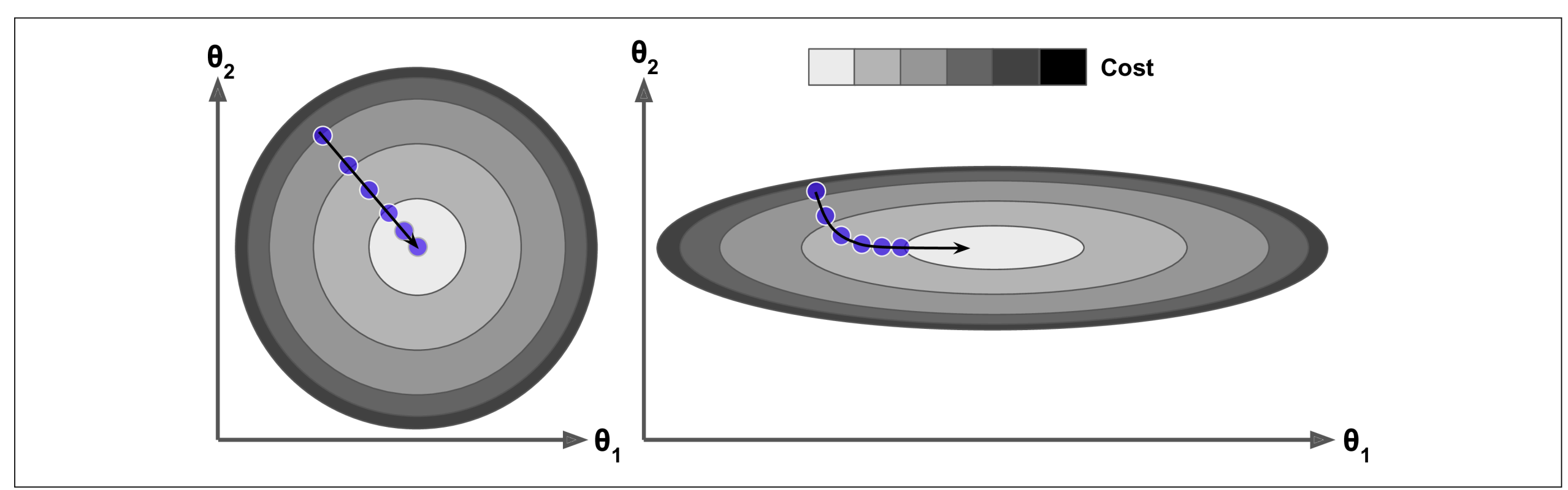
( Left: Scaled Features - Circular contours allow a direct path. | Right: Unscaled Features - Elongated contours cause a zigzag path. )
When using Gradient Descent, you should ensure that all features have a similar scale (e.g., using Scikit-Learn’s StandardScaler class), or else it will take much longer to converge.
Can we optimize too much? Yes. If we run Gradient Descent for too long on complex models, we risk Overfitting. We might find a solution that works perfectly for the training data but fails on new data. (We will cover this in Evaluation Metrics).
5. Parameter Initialization: Where do we start?
Gradient Descent is a journey. Every journey needs a starting point. The values we choose for $\theta$ at the very beginning can determine how fast (or if) we find the solution.
Setting all weights to 0.
When to use: Fine for Linear Regression (because it's a simple bowl). Danger: For Neural Networks, this causes "Symmetry," meaning all neurons learn the exact same thing, making the model useless.
Starting with small random numbers.
Benefit: Breaks symmetry. Each part of the model starts exploring a different part of the valley.
Using math formulas to pick random numbers based on the number of inputs.
👉 Deep Dive: Learn the Math behind He & Xavier
Sometimes we intentionally choose θ instead of random:
- a) Prior knowledge: If you have domain insight, you can start θ near expected values. This can significantly speed up convergence.
- b) Warm start: Use parameters from a previously trained model. Very common in iterative or online learning.